Skeletal Animation Looping with Autocorrelation
This is a bit of a fun post highlighting how some simple maths can be used to create great visual results. With some basic statistics, we can create looping skeletal animations from an input data set that contains non-exact loops. A typical example is a motion capture sampled run animation:
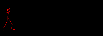
This is derived from the CMU Graphics Lab Motion Capture Database, which has been converted to BVH files by Bruce Hahne. I can load BVH files and dynamically retarget them to my animation rigs so that I never have to worry about changing animation rigs again (this is absolutely key to some of the features of my product and would have been immensely useful for the animation pipelines in many of my past games).
The first task is to center the animation on the origin to allow movement to be controlled by the game. Appropriate playback timing/blending and IK foot fixups are added after that. Many games simply strip the root bone offset from the animation but you lose a lot of animated weight transfer and bounce. I chose instead to send out a "rabbit" node that attempts to keep up with the moving skeleton via a fixed linear velocity, subtracting its position to get:
You can notice the three-and-a-bit steps the skeleton takes, the slow raising of the torso and the hard snap at the end when the animation ends. Somewhere in there is a two step loop that can be used to create a seamlessly looping animation. The tasks required are:
- Use auto/cross correlation to identify potential loop lengths in the animation.
- Search the animation using the loop lengths for start and end frames whose poses match.
- Cross-fade the beginning and end of the animation to smooth out the differences.
Statistics aren't my strong point so I would really appreciate any corrections to this post!
Cross Correlation
Given two discrete real data sets:
\[x = [ x_0, x_1, x_2, ..., x_n ]\]
\[y = [ y_0, y_1, y_2, ..., y_n ]\]
Correlation can give you a single number that tells you how similar these two data sets are. This number is generally called the correlation coefficient and can be calculated in a number of different ways, depending on what particular features of the data set you're interested in highlighting.
The most common coefficient appears to be the Pearson product-moment correlation coefficient. The coefficient is in the range -1 to 1, where 1 means there is a perfect linear relationship, 0 means there is no relationship and -1 means there is a negative linear relationship. A simple definition for a population is:
\[R(x,y) = \frac{1}{n} \sum\limits_{i=1}^n \frac{x(i) - m(x)}{s(x)} * \frac{y(i) - m(y)}{s(y)}\]
where \(m\) is the median and \(s\) is the standard deviation of the population.
Interestingly, this coefficient is independent of the unit of measurement: it can report 100% correlation between data sets that differ in scale or offset. For example, if set \(x\) recorded your age in months and set \(y\) recorded your height in inches at that age, it will be able to report any linear relationship (e.g. you get taller as you get older) with a correlation coefficient close to 1. This nice result is achieved by first of all centering each data set on its median and then transforming the set into units of its standard deviation.
Cross Correlation uses this basic tool to evaluate how similar two input data sets are when one of them is offset (or, time-lagged in the case of audio samples). Assuming the data sets are equal in length, for every sample in \(x\), the correlation coefficient is calculated with an offset version of \(y\):
\[xcorr(x, y)[n] = sum(x' [m] * y[m + n])\]
Here, \('\) is the complex conjugate. As we'll be dealing with real numbers, this can safely be ignored. You can use this for many things, like detecting the presence of one signal (or similar) somewhere within another, measuring tempo or even auto-tuning (yes, Mathematicians helped create our current generation of talentless musicians).
This leads to the following code:
double CrossCorrelate(const std::vector<double>& x, const std::vector<double>& y)
{
    // Assume data sets are the same size
    size_t size = x.size();
    assert(size == y.size());

    // Calculate mean and standard deviation of data sets
    double mx = mean(x);
    double my = mean(y);
    double sx = stddev(x);
    double sy = stddev(y);

    // Calculate correlation coefficient for each offset
    std::vector<double> Rxy(size);
    for (size_t i = 0; i < size; i++)
    {
        // First term can be pulled out of the inner loop
        double a = (x[i] - mx) / sx;

        double c = 0;
        for (size_t j = 0; j < size; j++)
        {
            // Second term is always offset by the constant 'i'
            // I'm choosing to wrap here whereas you can also zero-pad
            size_t ij = (i + j) % size;
            double b = (y[ij] - my) / sy;

            c += a * b;
        }

        Rxy[i] = c / size;
    }
}
Assuming the input data sets are the same size is not very useful in reality, however we don't need to do full cross correlation. With animation, we want to be able to detect loops within one dataset; essentially making \(x\) and \(y\) the same.
This is called Autocorrelation and it gets even better. Given that we're not interested in the unit-independent properties of cross correlation (we're comparing the same data set values), we can set the median to zero and standard deviation to one, leaving:
\[R(x,y) = \frac{1}{n} \sum\limits_{i=1}^n x(i) * y(i)\]
Application to Skeletal Animation
The data set we have is the rotation values of each bone in an animation for each frame (I'm ignoring scale as you don't generally get that from BVH data and translations are present only on root bones). We want to perform autocorrelation for each frame of the animation with a frame offset version of itself.
Autocorrelation above was defined in terms of scalar value multiplication, so an equivalent data type and multiplication operator needs to be defined for a single frame of animation. This can be achieved by using a vector of all bone rotations for a specific frame, combined with a vector dot product, which is effectively a projection of one frame onto another (result is max when all bones line up).
You can use the quaternion values directly or euler angles; it doesn't matter. We're not interested in the values themselves, we're just interested in how they relate to each other. I have found, though, that I'm getting better results using rotations that are relative to their parent bone, as opposed to object-space rotations.
This leads to the following code:
struct Anim
{
    size_t int nb_bones;
    size_t int nb_frames;

    // Just rotation data for all bones in all frames
    // size = nb_bones * nb_frames
    std::vector<quat> frame_data;
};

double DotProduct(
    const std::vector<quat>& x,
    const std::vector<quat>& y,
    size_t ox,
    size_t oy,
    size_t vector_size)
{
    // Dot product of two frame vectors. As they're just collections of rotation quaternions,
    // sum all quaternion dot products.
    double dp = 0;
    for (size_t i = 0; i < vector_size; i++)
    {
        quat q0 = x[ox + i];
        quat q1 = y[oy + i];
        dp += q0.x * q1.x + q0.y * q1.y + q0.z * q1.z + q0.w * q1.w;
    }
    return dp;
}


double Correlate(
    const Anim& anim,
    const std::vector<quat>& x,
    const std::vector<quat>& y,
    size_t frame_offset)
{
    double Rxy = 0;
    for (size_t i = 0; i < anim.nb_frames; i++)
    {
        // Shift and wrap to keep the inputs the same length
        size_t ox = i;
        size_t oy = (frame_offset + i) % anim.nb_frames;

        // Calculating the Pearson correlation co-efficient using mean of zero and stdev of 1
        Rxy += DotProduct(x, y, ox, oy, anim.nb_bones);
    }

    return Rxy / anim.nb_frames;
}

// Calculate the cross-correlation sequence using the same animation for both inputs (auto-correlation)
std::vector<double> Rxy(anim.nb_frames);
for (size_t i = 0; i < anim.nb_frames; i++)
    Rxy[i] = Correlate(anim, anim.frame_data, anim.frame_data, i);
When applied to the centered animation above, the sequence looks like this:
We're interested here in looking for the peaks of the graph, answering the question: other than at the start, where does the animation most look like itself? This is a standard local maximum search that starts off with computing the first derivative:
// We want to detect the local minimum/maximum points in the sequence, as periodicity
// estimates for the animation so calculate 1st derivative
std::vector<double> Rxy_df(anim.nb_frames);
for (size_t i = 1; i < Rxy.size(); i++)
    Rxy_df[i] = Rxy[i] - Rxy[i - 1];
leading to:
Local minima/maxima are located at the zero crossings and local maxima can be detected where the derivative is decreasing.
Searching for Start and End Frames
Just as autocorrelation in audio can only measure tempo and not tell you where specific beats are, this technique will only tell you potential lengths of the animation. Autocorrelation is a function of the signal, not a frame, so we will need to search the animation for start/end frames that match each other as closely as possible.
Beyond rotation similarity, we also want to ensure velocity/acceleration and general trajectory similarity. Given a potential start and end frame, we can determine a simple measure of similarity by summing squared distances within a set window. By walking through all possible start/end frames and keeping the smallest sum, we can get our best match.
This code is based on Benjy Cook's Python mocap tools for Blender, linked below.
double SqrDistance(
    const std::vector<quat>& x,
    const std::vector<quat>& y,
    size_t ox,
    size_t oy,
    size_t vector_size)
{
    double d = 0;
    for (size_t i = 0; i < vector_size; i++)
    {
        quat q0 = x[ox + i];
        quat q1 = y[oy + i];
        quat q = { q0.x - q1.x, q0.y - q1.y, q0.z - q1.z, q0.w - q1.w };
        d += q.x * q.x + q.y * q.y + q.z * q.z + q.w * q.w;
    }
    return d;
}

static const int WINDOW_SIZE = 5;
int best_fit_frame = -1;
size_t best_fit_length = 0;
double best_fit_sum = 0;

for (size_t i = 0; i < local_maxima.size(); i++)
{
    size_t length = local_maxima[i];

    // Precalculate distances between all possible start/end frames at this length
    std::vector<double> distance(anim.nb_frames - length);
    for (size_t j = 0; j < distance.size(); j++)
    {
        size_t ox = j * anim.nb_bones;
        size_t oy = (j + length) * anim.nb_bones;
        distance[j] = SqrDistance(anim.frame_data, anim.frame_data, ox, oy, anim.nb_bones);
    }

    // Search for the best start/end frame pair
    for (size_t j = WINDOW_SIZE; j < distance.size() - WINDOW_SIZE - 1; j++)
    {
        // Sum distances in local neighbourhood
        double sum = 0;
        for (size_t k = j - WINDOW_SIZE; k <= j + WINDOW_SIZE; k++)
            sum += distance[k];

        // Keep the best fit
        if (best_fit_frame == -1 || sum < best_fit_sum)
        {
            best_fit_frame = j;
            best_fit_length = length;
            best_fit_sum = sum;
        }
    }
}
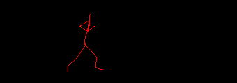
Using the best fit frame and length, the animation can then be clipped to give:
There are a few things to note about the result:
- The two step loop has been correctly identified.
- The start and end frames match pretty well: both leg and arm movement is almost seamless.
- There is a visible snap after the torso still rises for the duration of the animation.
Beyond employing better loop detection methods, this is really the best we can do without modifying the original animation. Even if we tried to look for better techniques, the chances of a single mocap shoot giving a perfectly loopable animation are minimal.
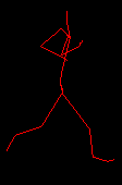
Cross-fading Around the Seam
The final simple part to this is to blend the last few frames in the animation so that they meet seamlessly with the frame at the start of the animation:
static const int BLEND_SIZE = 10;
for (size_t i = 0; i < BLEND_SIZE; i++)
{
    size_t offset = (anim.nb_frames - BLEND_SIZE + i) * anim.nb_bones;
    double t = (double)i / BLEND_SIZE;

    for (size_t j = 0; j < anim.nb_bones; j++)
    {
        const math::frame& dst = anim.frame_data[j];
        math::frame& src = anim.frame_data[offset + j];
        src = fLerp(src, dst, (float)t);
    }
}
A frame in my code base is an Affine Frame with vector position and quaternion rotation. I linearly interpolate both components based on their distance from the end of the animation (the quaternion lerp is normalised, as opposed to using slerp). This cleans up any small position differences in the hip bone.
The final result is pretty cool!
You can tweak the number of blend frames a little to get a smoother transition.
Conclusion
There is a whole bunch of stuff that you'll need to do to make this production-ready (loops within loops, signal filtering, artist pre/post input/modification, etc) but it this should be a good start.
Curiously, while debugging all my code for this I found that zero-crossings of the second differential (representing local minima of the first derivative) were giving good approximations to the start and end frame in animation loops:
If I start this specific animation at 15 and end it at 123, it loops just as well! I've not tested this on many data sets or dug into the maths further to see if there is anything to this, but it's an interesting avenue for future investigation.
Here's some links for further reading:
- Blender Mocap Tools - A great source code reference for stuff like this, written by Benjy Cook. (Python)
- Understanding Correlation - Online book hoping to shed some intuition on correlation.
- Autocorrelation for Tempo Estimation
- How do I implement Cross-correlation to prove two audio files are similar?